Saved: diffusion_pipeline_seed42.pngDATASCI 447 Lecture 28: The Omnimodal Frontier
Kevin McAlister
April 23, 2026
Administrative Stuff
Course Evals
Change: PS5 optional. If you want to do it, go for it. If not, no worries. Big reason - a lot of you are actually doing what you would’ve done in the problem set in your project. Use your colab budget for that instead.
Posters by tomorrow. Must be printed and dropped off in PAIS by 11:30 AM. If you want to present, make sure that you reach out to Ms. Charles to get on the schedule. A good way to show off the project!
Final project deliverables by May 5th at 11:59 PM. A final paper, website, etc. Must also submit a link to your replicable code Github. Make sure that your code is well documented and can be run by someone else. This is a requirement for the project. Make a nice README to explain what’s going on.
WHERE WE LEFT OFF
Last lecture we built the complete diffusion framework:
- Forward process: gradually add noise until data becomes \(\mathcal{N}(\mathbf{0}, \mathbf{I})\)
- Reverse process: a U-Net learns to predict and remove the noise, step by step
- Training: MSE on noise prediction — the simplest loss of any generative model
- Sampling: DDPM (stochastic) or DDIM (deterministic, 50 steps instead of 1000)
Two open questions remained:
- How do we control what the model generates?
- How do we make this practical for real images?
THE DIFFUSION FRAMEWORK IN 60 SECONDS
The core insight: instead of forcing a VAE encoder to match \(\mathcal{N}(\mathbf{0}, \mathbf{I})\) in one step (which creates prior holes), gradually walk from data to noise over \(T = 1000\) tiny steps, then learn to reverse the walk.
Forward process (fixed): add noise gradually until structure is destroyed.
\[\mathbf{x}_t = \sqrt{\bar{\alpha}_t}\,\mathbf{x}_0 + \sqrt{1 - \bar{\alpha}_t}\,\boldsymbol{\epsilon}\]
\(\bar{\alpha}_t\) is the signal survival rate — starts near 1 (clean), drops to 0 (pure noise). One formula jumps to any timestep.
Reverse process (learned): a U-Net predicts the noise \(\boldsymbol{\epsilon}_\theta(\mathbf{x}_t, t)\) at each step. Subtract the noise, take one step back toward clean data. Repeat \(T\) times.
THE TRAINING LOOP AND THE LOSS
The entire complex ELBO collapsed to:
\[L_{\text{simple}} = \mathbb{E}_{t,\,\mathbf{x}_0,\,\boldsymbol{\epsilon}}\left[\left\|\boldsymbol{\epsilon} - \boldsymbol{\epsilon}_\theta(\mathbf{x}_t, t)\right\|^2\right]\]
In plain English: pick a random image, add random noise at a random scale, train the network to predict what noise you added. MSE. That’s it.
The network acts as a compass — at any point in the noisy space, it points back toward the clean data manifold. Training at every noise scale means the compass works everywhere. No prior holes.
THE TRAINING LOOP AND THE LOSS

THE TRAINING LOOP AND THE LOSS
Saved: diffusion_pipeline_seed43.png
THE TRAINING LOOP AND THE LOSS
Saved: diffusion_pipeline_seed44.png
SAMPLING AND DDIM
DDPM sampling: start from pure noise, iteratively denoise over \(T\) steps. Each step: predict the noise, subtract most of it, add a tiny bit of fresh randomness. Stochastic — same starting noise gives different images.
DDIM sampling: deterministic variant. Same trained model, but no fresh noise at each step. Same starting noise always gives the same image.
Key advantage: DDIM tolerates skipped steps. 50 steps instead of 1000, no retraining needed. First big breakthrough in reducing the denoising tax.
Two open questions:
- How do we control what the model generates? \(\to\) conditioning and classifier-free guidance, next
- How do we make this practical for real images? \(\to\) latent diffusion, later today
THE CONDITIONING PROBLEM
Unconditional diffusion generates random images from the learned distribution. We want text-to-image. The network needs to know WHAT to generate, not just HOW to denoise.
We have CLIP text embeddings (big idea!) — a rich, semantically meaningful conditioning signal that lives in the same space as images (Lecture 26).
We need to inject those embeddings into the U-Net somehow so the noise prediction is steered by the text.
- How? With a mechanism you already know.
CROSS-ATTENTION CONDITIONING
Remember cross-attention from Lecture 22? Queries from one sequence, keys and values from another.
In the diffusion U-Net:
- Queries: U-Net feature maps (the image being denoised)
- Keys and Values: CLIP text embeddings (the conditioning signal)
Cross-attention layers are sandwiched between the conv/attention blocks at multiple resolutions in the U-Net. At every level of the hierarchy, the image features can “look at” the text to decide what content to generate.
In plain English: at each denoising step, the U-Net asks “what does the text want here?” and adjusts its noise prediction accordingly. The text steers the compass.
CROSS-ATTENTION CONDITIONING
Saved: unet_cross_attention.png
CROSS-ATTENTION CONDITIONING
Saved: diffusion_pipeline_conditioned_seed44.png
Look Where We Are
Look at what’s happening in that cross-attention layer:
- The U-Net architecture: from semantic segmentation
- The cross-attention mechanism: from transformers (L22)
- The CLIP text embeddings: from contrastive learning (L26)
- The denoising objective: from diffusion (L27)
Four separate threads from four different parts of the semester, meeting in one architectural component.
This is not a coincidence. It’s the payoff of building each piece carefully, understanding what it does, and recognizing where it fits in the larger system.
CLASSIFIER-FREE GUIDANCE
Cross-attention lets the model see the text. But in practice, the conditioning signal is too weak — generated images vaguely match the prompt but lack specificity.
The trick: train ONE model that sometimes sees the text and sometimes doesn’t. During training, randomly drop the text embedding (replace with a null embedding) with ~10-20% probability.
This gives us two modes from the same network:
- Conditional: \(\boldsymbol{\epsilon}_\theta(\mathbf{x}_t, t, \mathbf{c})\) — “denoise toward a dog”
- Unconditional: \(\boldsymbol{\epsilon}_\theta(\mathbf{x}_t, t, \varnothing)\) — “denoise toward… anything”
At inference, we amplify the difference between these two predictions.
THE GUIDANCE FORMULA
At inference, combine both predictions:
\[\hat{\boldsymbol{\epsilon}} = \boldsymbol{\epsilon}_\theta(\mathbf{x}_t, t, \varnothing) + w \cdot \left(\boldsymbol{\epsilon}_\theta(\mathbf{x}_t, t, \mathbf{c}) - \boldsymbol{\epsilon}_\theta(\mathbf{x}_t, t, \varnothing)\right)\]
In plain English: start with the unconditional prediction (“where does the data manifold generally live?”), then add an amplified version of the difference the conditioning makes.
THE GUIDANCE FORMULA
The guidance scale \(w\) controls how strongly the text steers generation:
- \(w = 1\): normal conditioning (often too weak)
- \(w = 7\text{-}15\): typical range for good text-to-image results
- \(w > 20\): oversaturated, artifacted, but very literal
This is the same idea as the negative prompts from the CLIP notebook — push toward what you want, push away from the generic baseline. Classifier-free guidance is the diffusion version of that exact technique.
WHY CLASSIFIER-FREE GUIDANCE WORKS
The difference \(\boldsymbol{\epsilon}_\theta(\mathbf{x}_t, t, \mathbf{c}) - \boldsymbol{\epsilon}_\theta(\mathbf{x}_t, t, \varnothing)\) isolates what the conditioning ADDS — the pure “dog-ness” direction in noise-prediction space, stripped of all the generic “image-ness” that both predictions share.
- Multiplying by \(w > 1\) amplifies this direction. You’re saying: “I don’t just want a slight lean toward dogs — I want DOGS, emphatically.”
Geometrically: the unconditional prediction points toward the center of the data manifold. The conditional prediction points toward the “dog” region. The guidance formula overshoots past “dog” to land deeper in the “dog” region than the model would naturally go.
- Without CFG, conditioned diffusion models produce vague, generic images.
THE PROBLEM WITH PIXEL-SPACE DIFFUSION
Running the U-Net 50 times on a 512×512×3 image is expensive. Each forward pass processes a 786,432-dimensional tensor through a billion-parameter network. 50 sequential evaluations, no parallelization across steps.
- The same problem we solved with VQ-VAE back in Lecture 19: raw pixels are too big. We need compression.
The lesson keeps repeating: don’t generate in pixel space. Generate in a compressed latent space and decode at the end.
LATENT DIFFUSION: THE STABLE DIFFUSION INSIGHT
Rombach et al. (2022): run diffusion in a compressed latent space instead of pixel space.
The architecture:
- A pretrained VAE compresses 512×512×3 images to 64×64×4 latents (48× fewer values)
- The U-Net operates on these small latents, not full images
- CLIP text encoder produces conditioning embeddings
- Cross-attention injects text conditioning into the U-Net
- After denoising, the VAE decoder maps latents back to pixel space
LATENT DIFFUSION: THE STABLE DIFFUSION INSIGHT
Saved: diffusion_pipeline_conditioned_seed44.png
THE SAME TRICK AS VQ-VAE
Same two-stage philosophy as DALL-E 1:
- Stage 1: learn a good compression (VAE / VQ-VAE)
- Stage 2: do generation in the compressed space (transformer / diffusion)
DALL-E 1: discrete latents + autoregressive transformer.
Stable Diffusion: continuous latents + iterative denoising.
- Same philosophy. Different generative mechanism. The continuous latents + diffusion combination produced dramatically better results.
Fun fact: the VQGAN paper (Esser, Rombach, Ommer, 2021) and the Stable Diffusion paper (Rombach et al., 2022) share authors. The same lab produced both the discrete-token path and the continuous-diffusion path — and then showed the world which one was better.
WHY THIS MADE DIFFUSION PRACTICAL
The numbers:
- Pixel-space diffusion on 512×512: each U-Net pass processes ~786K values
- Latent diffusion on 64×64×4: each U-Net pass processes ~16K values
- That’s 48× less computation per step
Plus fewer steps: DDIM + latent space means 20-50 steps instead of 1000.
WHY THIS MADE DIFFUSION PRACTICAL
The result: Stable Diffusion generates a 512×512 image in ~5 seconds on a consumer GPU. Pixel-space diffusion at equivalent quality would take minutes.
This is what made text-to-image generation accessible. Not a research demo — a product anyone could run on their own hardware. The open-source release of Stable Diffusion in August 2022 democratized image generation overnight.
ONE ARCHITECTURE
The complete Stable Diffusion stack,:
- VAE encoder/decoder (L17-19): compresses images to/from latent space
- Perceptual + adversarial losses (L19): make VAE reconstructions sharp
- U-Net with skip connections (L14, L27): the denoising backbone
- Self-attention in the U-Net (L22-23): global context at each resolution
- Cross-attention (L22): text conditioning injection point
- CLIP text encoder (L26): text \(\to\) aligned embedding
- InfoNCE / contrastive training (L26): how CLIP learned alignment
- Diffusion forward/reverse process (L27): the generative mechanism
- Noise prediction + simplified ELBO (L27): the training objective
- DDIM (L27): efficient deterministic sampling
- Classifier-free guidance (Lecture 20 + Today): amplified conditioning
EVERYTHING YOU’VE BUILT, IN ONE ARCHITECTURE
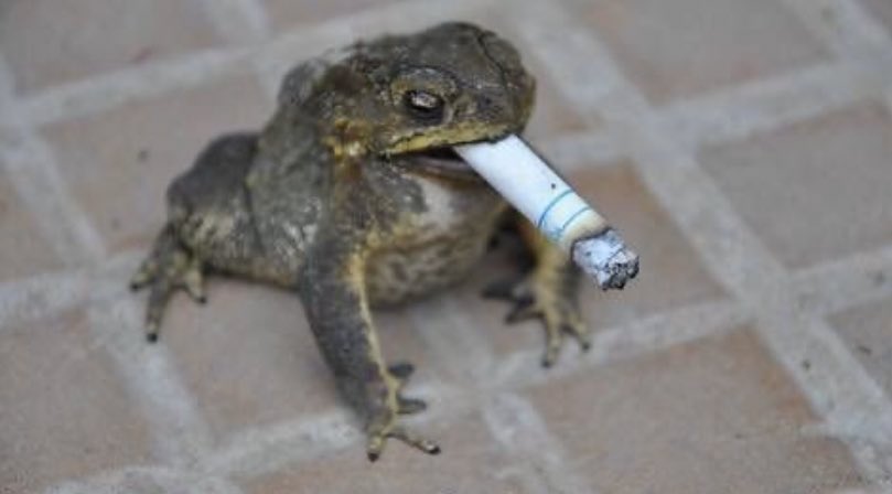
It’s 2026. You’ve used this.
THE FOUNDATION MODEL ARGUMENT
Stable Diffusion’s continuous latent space acts as a foundation model for visual generation.
Unlike VQ-VAE, which requires new codebook entries for new concepts, the continuous space can represent anything — including concepts it’s never explicitly seen.
“An astronaut riding a horse on Mars” works because the latent space is smooth and compositional, not because anyone trained on that specific image.
THE FOUNDATION MODEL ARGUMENT
One model, arbitrary prompts, infinite concepts. The continuous space + CLIP conditioning + diffusion creates a system that generalizes far beyond its training data.
This is the “everything in the same space” paradigm. The continuous latent space can do whatever we need it to — and that’s why pretrained multimodal models are the current foundation of generative AI.
EXTENSIONS THAT PROVE THE FOUNDATION
The Stable Diffusion base model spawned an entire ecosystem:
ControlNet: add new conditioning signals (edges, depth maps, poses) without retraining the base model. Just learn a new cross-attention pathway. The foundation’s representations are rich enough to support arbitrary conditioning.
LoRA for diffusion: apply low-rank adapters to the cross-attention weights. Train custom styles, characters, or concepts on a consumer GPU in minutes. Same technique from L25, applied to diffusion.
DreamBooth: personalize the model to generate specific subjects (your face, your pet) from 5-10 reference images. Fine-tune a tiny subset of parameters.
All of these work because the foundation is solid. You don’t rebuild the house — you add rooms.
THE DEATH OF “JUST AN LLM”
The term “large language model” is legacy. Modern frontier models are omnimodal foundation models.
GPT-4o processes text, images, audio, and video in one forward pass.
Gemini generates across modalities natively.
Claude analyzes images, writes code, and reasons about visual content.
These aren’t separate models stitched together. They’re single architectures that treat all modalities as tokens in a shared space.
The future isn’t “text models” and “image models” and “video models.” It’s one model that thinks in concepts and expresses them in whatever modality you ask for.
THE UNIVERSAL CONCEPT OF “DOG”
The word “dog,” a bark waveform, a photograph of a golden retriever, and a 3D mesh of a dog are no longer different modalities.
- They are the same mathematical coordinate in a shared latent space, aligned by contrastive learning (CLIP and its successors from L26).
This is the “everything in the same space” paradigm we’ve been building toward all semester. It’s not a metaphor — it’s the literal architecture of frontier AI systems.
The manifold hypothesis from Lecture 3. The representation learning thesis from Lecture 25. The contrastive alignment from Lecture 26. They were all building to this: one continuous space, all modalities, all concepts, all connected.
THE HYBRID ENGINE
Modern AI uses two complementary mechanisms:
Autoregressive transformers (GPT-style): for sequential reasoning — language, code, logic, planning. Generate one token at a time, each conditioned on everything before it.
Diffusion / flow models: for spatial generation — images, video, audio, 3D. Denoise all positions simultaneously, refining iteratively.
THE HYBRID ENGINE
These aren’t competing paradigms. They’re complementary tools that pass universal concepts back and forth through shared embedding spaces.
The LLM reasons about what to create. The diffusion model creates it. The representations flow seamlessly between them because they share the same latent geometry.
Generative ML is AI. What we call “AI” in 2026 is these two mechanisms, working together, operating in shared continuous spaces. That’s what this course taught you to understand.
THE HARDWARE WALL
The math we teach assumes infinite precision and unlimited memory. The engineering reality is different.
Modern frontier models are memory-bandwidth bound. The bottleneck isn’t compute speed — it’s how fast you can move weights from VRAM to compute cores. We’re using essentially all available VRAM in the world already.
I even struggle to implement real code examples on my machine. It’s a beast too.
I love my computer, but it can’t run a 70B-parameter model with 32GB of VRAM and 96GB of DDR5. The hardware wall is real.
THE HARDWARE WALL
Where do we go from here?
- Better silicon: HBM4, faster interconnects, more VRAM per chip. Slow (2-3 year cycles), expensive, power-hungry.
- Extreme quantization: run 70B models in 2-4 bit precision. Fits consumer VRAM, some quality loss. This is what makes local AI possible.
- Algorithmic efficiency: consistency models, flow matching, distillation. Do more with less compute.
Every deployment is a compromise between model quality and hardware constraints. Students entering industry will spend more time on these tradeoffs than on architecture design.
BREAKING THE DENOISING TAX
Diffusion’s Achilles heel: 20-50 sequential U-Net evaluations per image. Can we do better?
Consistency Models (Song et al., 2023): train a model that maps any noise level directly to the clean image in one step. Distill the iterative process into a single function. Near-diffusion quality at 1-4 steps.
Flow Matching (Lipman et al., 2023): instead of the noising/denoising Markov chain, learn a continuous flow field that transports noise to data along straight paths. Simpler math, often faster convergence. Stable Diffusion 3 uses flow matching internally.
The race toward \(O(1)\) generation — matching GANs’ speed with diffusion’s quality. We’re not there yet, but the gap is closing fast.
DIT: TRANSFORMERS EATING EVERYTHING
The U-Net is being replaced by Diffusion Transformers (DiT). Transformer Eat World
Patchify the noisy latent (exactly like ViT patches an image from L25), add timestep and conditioning embeddings, run through a standard transformer.
Why this matters: it’s the same architecture everywhere now.
- GPT for text generation
- ViT for visual representation
- DiT for visual generation
One architecture family, every modality, every task.
DIT: TRANSFORMERS EATING EVERYTHING
Sora (RIP in peace) is the concrete example: spacetime patches through a DiT, conditioned on text. Video generation using the same attention mechanism you learned in Lecture 23.
- The architectural distinction between “text models” and “image models” and “video models” is dissolving. It’s all transformers, all the way down.
NEW CAPABILITIES, NEW ETHICAL PROBLEMS
Every frontier we just discussed creates new ethical questions without settled answers:
Omnimodal generation: if one model produces photorealistic images, video, audio, and text — all indistinguishable from human-created content — how do we maintain trust in any media?
Foundation model access: training a frontier model costs $100M+. Is AI becoming a tool only available to the wealthiest institutions?
NEW CAPABILITIES, NEW ETHICAL PROBLEMS
Every frontier we just discussed creates new ethical questions without settled answers:
Consent and data: Stable Diffusion was trained on billions of images scraped from the web. Artists whose styles are reproducible never consented. Is this fair use? Courts are still deciding.
Alignment: as models become more capable, the gap between “what we asked for” and “what we meant” becomes more dangerous. CFG literally amplifies the model’s interpretation of your intent. What happens when that interpretation is wrong at scale?
Every technical advance creates new ethical surface area. The people best equipped to navigate these questions are the ones who understand the technology — which is now you.
NO QUICK ANSWERS
We don’t have good answers for most of these questions.
This is up to you — a new wave of technically gifted people who understand the tools, how they work, and why they work.
No quick answers. Just more and more thought needed — from people like you.
NOTICE WHAT WE NEVER DID
We never called this an “AI class.” The course is DATASCI 447. We talked about autoencoders, variational inference, attention mechanisms, contrastive learning, stochastic optimization, Markov chains.
We never invoked magic. We never said “the AI figured it out.” Every result — from VAE reconstructions to CLIP alignment to diffusion generation — followed from a loss function, a gradient, and enough data.
“AI” is a buzzword. What we actually studied is probabilistic machine learning — the mathematical framework for learning distributions from data and sampling from them.
- The fact that the results look like intelligence is a consequence of the math, not a replacement for it.
NOTICE WHAT WE NEVER DID
THIS IS A COP OUT. Don’t accept this logic that AI is “reasoning like a human”. You know better.
There’s a fine line between firing neurons and artificial systems.
Marketing garbage
NOTICE WHAT WE NEVER DID
The Blake Lemoine incident (Google, 2022) — A Google engineer publicly claimed LaMDA was sentient based on conversations where the model expressed feelings and fears. He was fired.
Stoked fear and more “anthropomorphizing AI” headlines. No technical basis for the claim. Just a human projecting onto a black box.
The “reasoning” we see is RHLF - match what the raters liked and don’t match what they didn’t.
Racism, sexism, and all.
NOTICE WHAT WE NEVER DID
When a model “refuses on moral grounds,” that’s a learned mapping from prompt patterns to refusal outputs that maximized reward during training. When it “expresses feelings,” it’s producing text that pattern-matches to emotional expression in its training corpus.
You know what’s inside the box. Next-token prediction. Noise prediction. Contrastive alignment. Variational bounds. None of these training objectives have a mechanism that produces subjective experience. The people making sentience claims generally don’t understand the training pipeline you just learned.
THE REAL LINEAGE
The work that powers “AI” in 2026 was enabled by decades of advances that nobody called AI at the time:
- Statistics: maximum likelihood estimation, Bayesian inference, the EM algorithm, variational methods — the conceptual foundations of every model we built
- Applied mathematics: optimization theory, differential equations, information theory, manifold geometry — the tools that make training possible
- Computer science: automatic differentiation, GPU computing, distributed systems — the engineering that makes scale possible
THE REAL LINEAGE
ChatGPT isn’t a breakthrough in “artificial intelligence.” It’s a breakthrough in applied Bayesian statistics running on very fast hardware.
- The transformer is a function approximator. Diffusion is a Markov chain. CLIP is a mutual information estimator. The ELBO is a variational bound. These aren’t AI concepts — they’re statistics concepts with good marketing.
THE ENGINE AND THE CHASSIS
The people who will make the next big contributions are the ones who understand what’s happening under the hood — not just the ones who can call .generate() on a pretrained model.
After this class, you understand the engine - not just “Machine go brr”
WHAT YOU NOW KNOW
After making it through this course, I’d argue you’re better informed than 90% of people in the ML world (loosely defined).
You can:
- Read and understand the original papers for every major architecture from the last decade
- Implement VAEs, VQ-VAEs, transformers, and fine-tuning pipelines from scratch
- Explain why diffusion works (not just that it works)
- Understand CLIP’s contrastive objective and its information-theoretic justification
- Fine-tune pretrained models with LoRA for arbitrary downstream tasks
- Critically evaluate claims in the AI hype cycle with actual technical knowledge
WHAT YOU NOW KNOW
Most people in “AI” can use APIs. You understand what the APIs are doing.
This is largely due to my very detailed slides (which is actually my book project!)
WHAT I TRIED THIS YEAR
This is the first time I’ve taught the course this way.
The bet: start with probabilistic ML and Bayesian foundations before touching neural networks. Build the statistical scaffolding first, then show that every modern architecture is a special case.
WHAT I TRIED THIS YEAR
The arc: probability \(\to\) likelihood \(\to\) Bayesian inference \(\to\) “the stupid integral” \(\to\) curse of dimensionality \(\to\) PCA \(\to\) neural networks as nonlinear PCA \(\to\) CNNs \(\to\) the transfer paradigm \(\to\) generation from VAEs \(\to\) transformers \(\to\) autoregressive generation \(\to\) richest representations driving generation \(\to\) CLIP for omnimodal alignment \(\to\) the actual modern pipeline.
Every step designed to feel like a natural extension of the previous one. Not “here’s a new architecture to memorize” but “here’s the next question that the previous answer forces us to ask.”
WHAT I THINK WORKED
The Bayesian foundations were in the right place. By the time we hit the ELBO in VAEs, you already knew what marginal likelihood was and why the integral is intractable. That’s a 10-lecture head start over most ML courses.
The representation learning thread — PCA to autoencoders to CNNs to ViTs — gave the whole semester a spine. Every lecture was about the same question: how do we find good representations?
The generative arc from VAEs through CLIP to diffusion told one continuous story. Each model solved a specific limitation of the previous one.
WHAT I’M GOING TO FIX
The first 6 lectures were too aggressive. Figure out the right pacing.
The Bayesian inference lecture — marginal likelihood, Occam’s razor, intractability — tried to do too much in one sitting. Next year: split it, slow down, let the ideas breathe.
Teaching is a generative model. Each year is a training step. The loss is decreasing.
WHERE TO GO FROM HERE
If you want to go deeper:
Read the original papers. You now have the vocabulary to understand them. Start with “Attention Is All You Need,” the CLIP paper, and the DDPM paper.
Build something. Fine-tune a model for a problem you care about. Train a small diffusion model from scratch. Contribute to an open-source project.
Take follow-up courses. Deep reinforcement learning, probabilistic graphical models, information theory, optimization theory.
The field is moving incredibly fast. What you learned this semester is the foundation. The specific architectures will evolve, but the underlying principles — representation learning, variational inference, attention, contrastive alignment — will remain.
The END
We started the semester with logistic regression.
We ended with Stable Diffusion.
The intellectual distance between those two is vast, but every step was a reasonable incremental extension of what came before.
The END
That’s the real lesson: complex systems are built from simple, well-understood parts.
Understanding those parts — not just using them, but truly understanding them — is what separates the people who advance the field from the people who use what the field produces.
The END
You now understand the parts.
Go build something extraordinary.
And listen to the playlist that covers all of the songs that I never really found a place to link within our lectures (explicitly or hidden hint hint).
DATASCI447 Playlist (My Gift To You - You’re Welcome)